機械学習のモデルを作るときは、とりあえずXGBoostにしとけばよいでしょっていうぐらい、XGBoostが優秀です。ただし、XGBoostはある程度の精度のモデルを何も考えずに構築できる反面、他の機械学習モデルよりは実行時間が長くなります。モデルの学習時間が長くなると、ハイパーパラメータの探索回数を制限せざる負えなくなり、モデルの精度にも関わってきてしまいます。
学習データのデータサイズが大きくなるときは、すべてのデータに意味があるというよりは、ほぼ0の値で埋まっているようなスパース(疎)なデータになっていることが多いです。予測モデルにとっては、0列が多いことで精度が上がることはなく、実行時間がその分かかってしまうためよくないです。
そこで今回は、スパース(疎)なデータを非スパースなデータに変換して学習させることで、学習時間の高速化を行います。これによりモデルの予測精度が下がることはないということも確かめます。本記事のコードを実行すると、以下のようにXGBoostの高速化ができます。今回のコードはこちらにあります。

今回使用するデータ
まずは今回使用するモジュールを先にインポートし、扱うデータの説明をします。スパースなデータを非スパースなデータに変換するために、scipyモジュールを使います。
モージュルのインポートと準備
from pathlib import Path
import sys
import scipy
import numpy as np
import pandas as pd
import time
import matplotlib.pyplot as plt
import seaborn as sns
import xgboost as xgb
from sklearn.datasets import make_classification
from sklearn.model_selection import train_test_split, StratifiedKFold

result_dir_path = Path('result')

if not result_dir_path.exists():
    result_dir_path.mkdir(parents=True)
使用するデータとデータのスパース化
今回の実験で扱うデータは、sklearn.datasets.make_classification 関数を使って作ります。これ自体は特に何を使っても大丈夫でしょう。大事なのは、このベースデータを使ってスパースなデータに変換することです。とはいっても、値が0のみの列データを追加するだけですが。
X_data, y_data = make_classification(
n_classes=4,
n_samples=10,
n_features=6,
n_clusters_per_class=1,
n_informative=4,
random_state=42
)
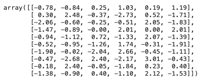
X_data
y_data
![]()
上を見てもらえば分かる通り、機械学習モデルの入力データである行列と出力データであるベクトルができています。この入力用データに0列のデータを追加することで、データをスパース化させます。

データの非スパース化
今回の核心であるスパースなデータの非スパース化処理を実践します。実は非常に簡単です。これをやるために、まずはスパースなデータを作成します。
X_data, y_data = make_classification(
    n_classes=4,
    n_samples=10,
    n_features=6,
    n_clusters_per_class=1,
    n_informative=4,
    random_state=42
)

data = pd.DataFrame(
    X_data,
    columns=['X' + str(i + 1) for i in range(X_data.shape[1])]
)

new_0_col = 10

data = pd.concat([
    data,
    pd.DataFrame(
        np.zeros((data.shape[0], new_0_col)),
        columns=['X' + str(i + data.shape[1] + 1) for i in range(new_0_col)]
    )
], axis=1)
data
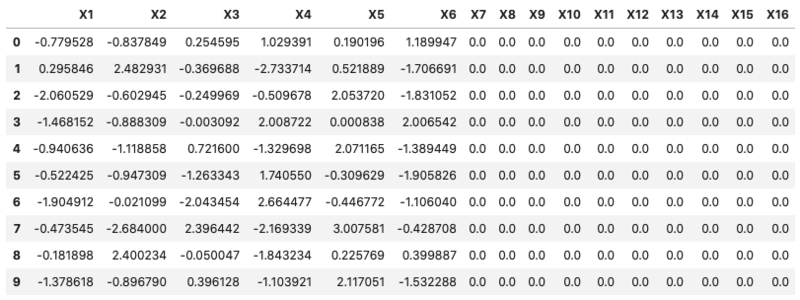
変数「new_0_col」で指定した分の値が0の列をベースデータに追加しています。スパースなデータになったので、このデータを非スパース化します。そのために、scipyのcsr_matrix 関数を使います。この関数を使えば、ワンライナーで非スパース化できるのです。
data_sparsed = scipy.sparse.csr_matrix(data)
以上で終わりです。3分クッキングよりも短いですね。この非スパース化したデータの中身を見てみます。
data_sparsed.data
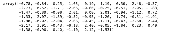
上のベクトルは、スパース化する前の行列データを0行目から順に格納していっており、値が0の場合は省かれています。これにより非スパースなベクトルになっているのです。ただこのデータだけでは、各値の元々の行列の場所がわからないため、元の行列に戻せなくなります。そこで、スパース化したデータでは、各値の元の列のインデックスベクトルとそのイデックスベクトルのどこまでが何行目かのデータも持っています。
data_sparsed.indices

上のベクトルは、値ベクトルに対応しており、それぞれの値ベクトルがもとの行列の何列目かを保持しています。
data_sparsed.indptr
![]()
このベクトルは行を管理しており、元の行列の何行目かを、列インデックスベクトルの添字で表しています。例えば、元の行列0行目に対応する列インデックスは data_sparsed.indptr[0] ~ data_sparsed.indptr[1] の範囲であり、元の行列の0行目の値を持ってくる場合は、以下のコードになります。
data_sparsed.data[data_sparsed.indices[
    data_sparsed.indptr[0]: data_sparsed.indptr[1]
]]
![]()
これでデータの非スパース化は完成です。次からは、非スパース化データにすることで、XGBoostの学習時間が短くなるのかを見ていきます。スパース化/非スパース化による学習時間を比較するために、先にスパースなデータを使いXGBoostの学習時間を計測します。
スパースなデータでのXGBoostの学習時間の計測
非スパースなデータの作り方がわかったので、そのデータを使うことにより学習時間が短くなるかを確認したいのですが、先にスパースなデータでXGBoostの学習時間がどれだけかかるかを見ておきます。以下のコードでは、ベースデータを10,000と20,000、追加する0列の件数を [0, 10, 100, 1000, 10000] とし、それぞれの設定で交差検証法により複数回学習しています。交差検証法を使っているのは、それぞれの設定での処理時間を平均値にして比較するためです。
n_splits = 5

cv_results = []
for n_samples in [10000, 20000]:

    X_data, y_data = make_classification(
        n_classes=10,
        n_samples=n_samples,
        n_features=100,
        n_clusters_per_class=1,
        n_informative=4,
        random_state=42
    )

    X_data = pd.DataFrame(X_data, columns=['x' + str(i + 1) for i in range(X_data.shape[1])])

    for n_new_0_col in [0, 10, 100, 1000, 10000]:

        X_data_ = pd.concat([
            X_data,
            pd.DataFrame(
                np.zeros((X_data.shape[0], n_new_0_col)),
                columns=['x' + str(X_data.shape[1] + i + 1) for i in range(n_new_0_col)]
            )
        ], axis=1)

        X_train, X_test, y_train, y_test = train_test_split(
            X_data_, y_data, test_size=0.3, random_state=42, shuffle=True
        )

        kf = StratifiedKFold(n_splits=n_splits)

        loop = 1
        for indexes_train, indexes_valid in kf.split(X_train, y_train):

            X_train_cv = X_train.iloc[indexes_train]
            y_train_cv = y_train[indexes_train]
            X_valid_cv = X_train.iloc[indexes_valid]
            y_valid_cv = y_train[indexes_valid]

            start_time = time.time()
            model = xgb.XGBClassifier(random_state=42, use_label_encoder=False)
            model.fit(
                X_train_cv,
                y_train_cv,
                early_stopping_rounds=30,
                eval_set=[(X_valid_cv, y_valid_cv)],
                eval_metric='mlogloss',
                verbose=0
            )
            end_time = time.time()

            score = model.score(X_test, y_test)
            print('Samples: {}, New 0 Col: {}, [{}/{}], Score: {:.0f}%, {:.0f}s'.format(
                n_samples, n_new_0_col, loop, n_splits, score * 100,
                end_time - start_time
            ))

            cv_results.append([n_samples, n_new_0_col, loop, end_time - start_time, score])
            loop += 1

cv_results = pd.DataFrame(
    cv_results,
    columns=['n_samples', 'new_n_0_col', 'loop', 'elapsed_time', 'score']
)
cv_results.to_csv(result_dir_path.joinpath('model_result_sparse.csv'), index=False)
cv_results
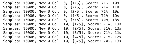
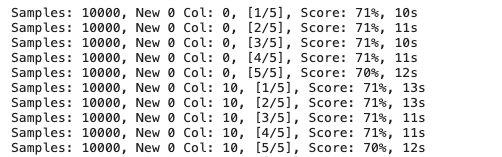
上のコードはそこまで難しくないと思います。pd.concatにより、指定した件数の0列を追加してデータをスパース化し、交差検証法により複数回の学習をしています。筆者の環境では、ベースデータ20,000件、追加する0列のデータ10,000件にすると、学習時間は688秒でした。結構な処理時間でしたね。
次に非スパース化したデータを使ったXGBoostの学習時間を見ていきます。
非スパースなデータでのXGBoostの学習時間の計測
スパースなままのデータでXGBoostを学習させると、結構な時間がかかることが確認できました。同じ設定で、スパースなデータを非スパース化して学習させて、処理時間を測定します。
n_splits = 5

cv_results = []
for n_samples in [10000, 20000]:

    X_data, y_data = make_classification(
        n_classes=10,
        n_samples=n_samples,
        n_features=100,
        n_clusters_per_class=1,
        n_informative=4,
        random_state=42
    )

    X_data = pd.DataFrame(X_data, columns=['x' + str(i + 1) for i in range(X_data.shape[1])])

    for n_new_0_col in [0, 10, 100, 1000, 10000]:

        X_data_ = pd.concat([
            X_data,
            pd.DataFrame(
                np.zeros((X_data.shape[0], n_new_0_col)),
                columns=['x' + str(X_data.shape[1] + i + 1) for i in range(n_new_0_col)]
            )
        ], axis=1)

        X_train, X_test, y_train, y_test = train_test_split(
            X_data_, y_data, test_size=0.3, random_state=42, shuffle=True
        )

        kf = StratifiedKFold(n_splits=n_splits)

        loop = 1
        for indexes_train, indexes_valid in kf.split(X_train, y_train):

            X_train_cv = X_train.iloc[indexes_train]
            y_train_cv = y_train[indexes_train]
            X_valid_cv = X_train.iloc[indexes_valid]
            y_valid_cv = y_train[indexes_valid]

            start_time = time.time()
            model = xgb.XGBClassifier(random_state=42, use_label_encoder=False)
            model.fit(
                scipy.sparse.csr_matrix(X_train_cv),
                y_train_cv,
                early_stopping_rounds=30,
                eval_set=[(scipy.sparse.csr_matrix(X_valid_cv), y_valid_cv)],
                eval_metric='mlogloss',
                verbose=0
            )
            end_time = time.time()

            score = model.score(scipy.sparse.csr_matrix(X_test), y_test)
            print('Samples: {}, New 0 Col: {}, [{}/{}], Score: {:.0f}%, {:.0f}s'.format(
                n_samples, n_new_0_col, loop, n_splits, score * 100,
                end_time - start_time
            ))

            cv_results.append([n_samples, n_new_0_col, loop, end_time - start_time, score])
            loop += 1

cv_results = pd.DataFrame(
    cv_results,
    columns=['n_samples', 'new_n_0_col', 'loop', 'elapsed_time', 'score']
)
cv_results.to_csv(result_dir_path.joinpath('model_result_non_sparse.csv'), index=False)
cv_results
上のコードにおいて、スパースなデータを使った実験と変わったところは、「csr_matrix」関数を使いデータを非スパース化してから、XGBoostを学習させていることです。筆者の環境では、ベースデータ20,000、追加する0列のデータ10,000での学習時間は、74秒でした。つまり、非スパース化することで9倍も短縮されています。
実験結果をグラフ化
上記の実験で、データを非スパース化することで、XGBoostの学習時間の短縮を確認できました。このことが視覚的に裏付けるために、グラフ化して見てみましょう。
target_data = pd.concat([
    pd.read_csv(result_dir_path.joinpath('model_result_non_sparse.csv')).assign(
        category='non_sparse'
    ),
    pd.read_csv(result_dir_path.joinpath('model_result_sparse.csv')).assign(
        category='sparse'
    )
], axis=0)

plot_data = target_data.groupby(['category', 'new_n_0_col', 'n_samples']).agg({
    'elapsed_time': ['mean', 'std'], 'score': ['mean', 'std']
})
plot_data.columns = ['elapsed_time_mean', 'elapsed_time_std', 'score_mean', 'score_std']
plot_data.reset_index(inplace=True, drop=False)

g = sns.relplot(
    data=plot_data.assign(new_n_0_col=lambda x: x.new_n_0_col.astype(str)),
    x='new_n_0_col',
    y='elapsed_time_mean',
    hue='category',
    col='n_samples',
    kind='line',
    marker='o',
    markersize=10
)
g.fig.suptitle('スパース/非スパースデータによるXGBoostの学習時間', fontsize=18, y=0.98, weight='bold')
g.fig.set_figwidth(12)
g.fig.set_figheight(6)
for ax in g.axes.flat:
    ax.set_xlabel('値0の列追加件数', size=14)
    ax.set_title(ax.get_title(), size=14)
g.set_ylabels('')

leg = g._legend
leg.set_bbox_to_anchor([0.17, 0.8])

for i, ax in enumerate(g.axes.flat):
    for tick in ax.get_yticks()[1:-1]:
        ax.axhline(tick, alpha=0.1, color='grey')

plt.tight_layout()
plt.savefig(result_dir_path.joinpath('model_result_sparse_vs_non_sparse_slapsed_time.png'), dpi=300)

上のグラフを見て分かる通り、スパースなデータは非スパースなデータに比べて、値0の列が増えるに連れ、学習時間が顕著に増加しています。スパースなままXGBoostを学習させることは、多大な時間を浪費するのです。
非スパースにより学習時間が短くなることが証明されましたが、これにより予測精度が落ちていたら元も子もありません。そこで、予測精度が影響を受けているかを確認しておきます。
result = pd.pivot_table(
    data=plot_data[['n_samples', 'category', 'new_n_0_col', 'score_mean', 'score_std']],
    index=['n_samples', 'new_n_0_col'],
    columns='category'
)
result
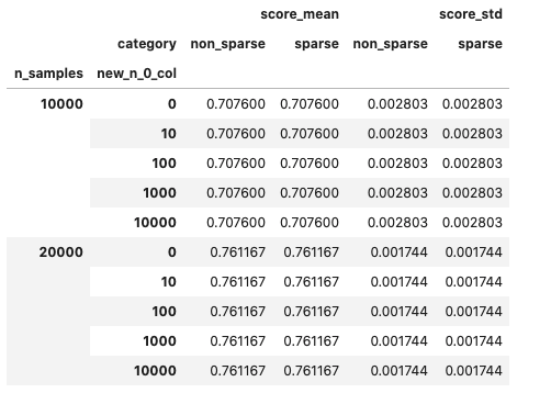
予測精度に変化はありません。つまり、スパースなデータのままXGBoostを学習させることは、損しかないと言えそうです。
終わりに
今回はXGBoostというか機械学習における学習時間の高速化の話をしました。ワンライナーで学習時間が大幅に変わるので、やらない手はないと思います。今回取り上げませんでしたが、XGBoostのハイパーパラメータの調整や機械学習の精度向上に関しては、以下の本が参考になりました。
