テキストから示唆を作り出すテキストマイニングの一つとして、今回は文章から共起ネットワークを作ります。共起ネットワークは、同時に出現する単語の組み合わせをエッジで繋ぎ、単語間の関係をネットワークで表したものです。これにより、文章内の単語の関連性を可視化できます。
今回は、Pythonの「networkx」を使って、共起ネットワークを実装します。今回の記事で最終的に出来上がった共起ネットワークは以下になりました。

今回の記事のコードはここに置いてあります。
データの準備
共起ネットワークを描くためには、テキストを文章を1区切りとして分割し、文章ごとに同時に出現する単語の組み合わせリストを作る必要があります。これを愚直に実行していきますが、そもそもデータが無いと何も始まらないので、データを用意し、ノイズを取り除きます。
必要モジュールのインポート
必要モジュールを一気インポートします。今回での注目モジュールはやはり「networkx」ですね。
from pathlib import Path
import re
import collections
import pandas as pd
import MeCab
import mojimoji
import neologdn
import unicodedata
import itertools
import networkx as nx
import matplotlib.pyplot as plt

data_dir_path = Path('data')
result_dir_path = Path('result')

if not result_dir_path.exists():
    result_dir_path.mkdir(parents=True)
データの取得と加工
今回使用するデータは、青空文庫 Aozora Bunkoにある福沢諭吉の『学問のすすめ』です。すでにテキストファイル化したものは、ここに置いてあります。このテキストファイルから共起ネットワークを作るのですが、テキストはノイズが多いので前処理が必要になります。今回は、前処理のコードをサックと記載するだけなので、詳しくはこの記事を御覧ください。
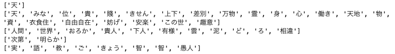
以下のコードでは、取得したテキストを「。」で分割し、分割した文章から名詞だけを抽出しています。
def get_stopword_lsit(write_file_path):

    if not write_file_path.exists():
        url = 'http://svn.sourceforge.jp/svnroot/slothlib/CSharp/Version1/SlothLib/NLP/Filter/StopWord/word/Japanese.txt'
        urllib.request.urlretrieve(url, write_file_path)

    with open(write_file_path, 'r', encoding='utf-8') as file:
        stopword_list = [word.replace('\n', '') for word in file.readlines()]

    return stopword_list


def get_noun_words_from_sentence(sentence, mecab, stopword_list=[]):
    return [
        x.split('\t')[0] for x in mecab.parse(sentence).split('\n') if len(x.split('\t')) > 1 and \
         '名詞' in x.split('\t')[3] and x.split('\t')[0] not in stopword_list
    ]


def split_sentence(sentence, mecab, stopword_list):
    sentence = neologdn.normalize(sentence)
    sentence = unicodedata.normalize("NFKC", sentence)
    words = get_noun_words_from_sentence(
        sentence=sentence, mecab=mecab, stopword_list=stopword_list
    )
    words = list(map(lambda x: re.sub(r'\d+\.*\d*', '0', x.lower()), words))
    return words

with open(data_dir_path.joinpath('gakumonno_susume.txt'), 'r', encoding='utf-8') as file:
    lines = file.readlines()

sentences = []
for sentence in lines:
    texts = sentence.split('。')
    sentences.extend(texts)

mecab = MeCab.Tagger('-Ochasen')

stopword_list = get_stopword_lsit(data_dir_path.joinpath('stopword_list.txt'))

noun_sentences = []
for sentence in sentences:
    noun_sentences.append(
        split_sentence(sentence=sentence, mecab=mecab, stopword_list=stopword_list)
    )

for words in noun_sentences[:5]:
    print(words)
共起ネットワークを作るので一語しかない文章を取り除き、更にノイズとなる「見出し」の単語が含まれている文章も削除しています。
noun_sentences = list(filter(lambda x: len(x) > 1 and '見出し' not in x, noun_sentences))
これでデータの取得と前処理は完了です。
共起ネットワークのためのデータ整形
今回作る共起ネットワークは、同じ文章に出現する単語を共起としているため、文章内での単語の組み合わせを作ります。
combination_sentences = [list(itertools.combinations(words, 2)) for words in noun_sentences]
combination_sentences = [[tuple(sorted(combi)) for combi in combinations] for combinations in combination_sentences]
tmp = []
for combinations in combination_sentences:
    tmp.extend(combinations)
combination_sentences = tmp
combination_sentences[:5]
![]()
エッジの重みJaccard係数
共起ネットワークでは、共起した単語の組み合わせをエッジでつなぎます。そのときに、エッジに対して重みを与え、その重みに応じてエッジの太さを変えることで、テキストマイニングでの示唆をより得やすくなります。
今回はその重みとして、Jaccard係数を使います。Jaccard係数をサクッと説明すると、和集合の数に対して積集合の数の割合です。詳しくは【技術解説】集合の類似度(Jaccard係数,Dice係数,Simpson係数)が参考になります。Jaccard係数は以下の式です。
積集合の個数が単語の組合せの個数を表し、それを和集合の数で割ることで、一方しか多く現れていない組合せのJaccard係数が大きくならないようにしています。ただ、和集合の数を求めるのは計算コストが高いので、和集合の数を求めるための基本式である次式を利用します。
実際のコードはこちらになります。
def make_jaccard_coef_data(combination_sentences):

    combi_count = collections.Counter(combination_sentences)

    word_associates = []
    for key, value in combi_count.items():
        word_associates.append([key[0], key[1], value])

    word_associates = pd.DataFrame(word_associates, columns=['word1', 'word2', 'intersection_count'])

    words = []
    for combi in combination_sentences:
        words.extend(combi)

    word_count = collections.Counter(words)
    word_count = [[key, value] for key, value in word_count.items()]
    word_count = pd.DataFrame(word_count, columns=['word', 'count'])

    word_associates = pd.merge(
        word_associates,
        word_count.rename(columns={'word': 'word1'}),
        on='word1', how='left'
    ).rename(columns={'count': 'count1'}).merge(
        word_count.rename(columns={'word': 'word2'}),
        on='word2', how='left'
    ).rename(columns={'count': 'count2'}).assign(
        union_count=lambda x: x.count1 + x.count2 - x.intersection_count
    ).assign(jaccard_coef=lambda x: x.intersection_count / x.union_count).sort_values(
        ['jaccard_coef', 'intersection_count'], ascending=[False, False]
    )

    return word_associates

jaccard_coef_data = make_jaccard_coef_data(combination_sentences)

jaccard_coef_data.head(10)
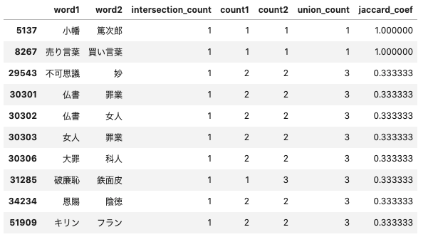
Jaccard係数を算出できましたが、実行結果をよく見ると、Jaccard係数が高い単語の組み合わせは、単語の出現回数が少ないものが多いようです。まぁ、単語の組み合わせの強さを見るためには必要なデータですが、文章全体を把握するという観点では、ノイズかもしれません。共起ネットワークを作る際は、単語の出現回数を考慮したほうが良いでしょう。
Jaccard係数の分布
エッジの重みであるJaccard係数を算出できたので、どの値が多いのかの分布を見てみます。
group_values = [0, 0.01, 0.02, 0.04, float('inf')]

plot_data = jaccard_coef_data.copy()
plot_data['group_num'] = 0
group_names = []
for i in range(len(group_values) - 1):

    plot_data['group_num'] = plot_data.apply(
        lambda x: i + 1 if group_values[i] <= x['jaccard_coef'] and x['jaccard_coef'] < group_values[i + 1] else x['group_num'],
        axis=1
    )
    group_names.append((group_values[i], group_values[i + 1]))

plot_data = plot_data.groupby('group_num')['jaccard_coef'].count().reset_index().rename(
    columns={'jaccard_coef': 'n_combi'}
).assign(rate=lambda x: x.n_combi / x.n_combi.sum()).assign(
    rate_cumsum=lambda x: x.rate.cumsum()
)
plot_data = pd.concat([
    pd.DataFrame(group_names, columns=['jaccard_lower', 'jaccard_upper']),
    plot_data
], axis=1)

plot_data
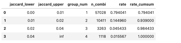
Jaccard係数が0.01未満である単語の組み合わせが多いですね。Jaccard係数が低いということは、様々な組み合わせに使われている単語ということになるので、注目すべき単語ではないです。なので、共起ネットワークを作る際には、Jaccard係数の下限値を設定したほうが良さそうです。
共起ネットワークの作成
これまでの処理でネットワークを構築するための準備が完了したので、実際に共起ネットワークを作ります。処理の流れは以下の通りです。
- ネットワークのインスタンスを作る
- ノードを追加
- エッジを追加
- 孤立ノードの削除
- ネットワークインスタンスへの書込み
今回はノードの大きさと色をPageRankの値に応じて変えています。PageRankの説明は次数中心性からPageRankからまた次数中心性 - でかいチーズをベーグルするが参考になります。ざっくりいうと、他のノードからの遷移数が多いノードの値が高くなります。下記のコードでは、日本語に対応するために fontfamily を設定するようにしています。何を設定したらよいかわからない方は、matplotlibで日本語 - Qiitaが参考になると思います。
def plot_network(
    data, edge_threshold=0., fig_size=(15, 15),
    fontfamily='Hiragino Maru Gothic Pro', fontsize=14,
    coefficient_of_restitution=0.15,
    image_file_path=None
):

    nodes = list(set(data['node1'].tolist() + data['node2'].tolist()))

    plt.figure(figsize=fig_size)

    G = nx.Graph()
    # 頂点の追加
    G.add_nodes_from(nodes)

    # 辺の追加
    # edge_thresholdで枝の重みの下限を定めている
    for i in range(len(data)):
        row_data = data.iloc[i]
        if row_data['weight'] >= edge_threshold:
            G.add_edge(row_data['node1'], row_data['node2'], weight=row_data['weight'])

    # 孤立したnodeを削除
    isolated = [n for n in G.nodes if len([i for i in nx.all_neighbors(G, n)]) == 0]
    for n in isolated:
        G.remove_node(n)

    # k = node間反発係数
    pos = nx.spring_layout(G, k=coefficient_of_restitution)

    pr = nx.pagerank(G)
    # nodeの大きさ
    nx.draw_networkx_nodes(
        G, pos, node_color=list(pr.values()),
        cmap=plt.cm.Reds,
        alpha=0.7,
        node_size=[60000*v for v in pr.values()]
    )

    # 日本語ラベル
    nx.draw_networkx_labels(G, pos, font_size=fontsize, font_family=fontfamily, font_weight="bold")

    # エッジの太さ調節
    edge_width = [d["weight"] * 100 for (u, v, d) in G.edges(data=True)]
    nx.draw_networkx_edges(G, pos, alpha=0.4, edge_color="darkgrey", width=edge_width)

    plt.axis('off')
    plt.tight_layout()

    if image_file_path:
        plt.savefig(image_file_path, dpi=300)

n_word_lower = 50
edge_threshold=0.025
plot_data = jaccard_coef_data.query(
    'count1 >= {0} and count2 >= {0}'.format(n_word_lower)
).rename(
    columns={'word1': 'node1', 'word2': 'node2', 'jaccard_coef': 'weight'}
)

plot_network(
    data=plot_data,
    edge_threshold=edge_threshold,
    fig_size=(10, 10),
    fontsize=9,
    fontfamily='Hiragino Maru Gothic Pro',
    coefficient_of_restitution=0.08,
    image_file_path=result_dir_path.joinpath('co_occurence_network.png')
)
共起ネットワークを見ると、いくつかの塊ができていることがわかります。単語のつながりが多いのは「官許」という単語です。文章全体を通して「官」に関連したことが重要であろうことが伺えます。エッジの太さを見ると、「変動」と「戦争」がほかと比べて太く、激動の時代に書かれた文章であることが伝わってきますね。
まだまだ示唆を読み取れそうな気がしますが、不要な単語も見られるため、追加の前処理が必要そうです。ただ、一定の示唆は得られそうであり、テキストマイニングの手法としては有効ですね。
終わりに
今回、共起ネットワークにより文の単語の組み合わせから、文全体の趣旨を読み取ることに挑戦しました。テキストマイニングとは別に、ネットワークの構成という話は奥が深く、勉強しがいがあります。ネットワークの構造に関して更に深ぼりをしたい方はこちらの本がおすすめです。
")